An Analysis of Surface Temperature Changes for Urban Green Space using Unmanned Aerial Vehicles
Article information

Abstract
Background and objective
The urban heat island (UHI) effect is recognized as a representative environmental problem that occurs in cities in summer. This study aimed to quantitatively determine the surface temperature (ST) of UGSs using high-resolution images taken by an unmanned aerial vehicle (UAV), and analyze time-series changes in ST according to spatial characteristics (conifers, deciduous trees, shrubs, grass, metal sculptures, pavements).
Methods
In this study, ST data of UGSs were established and acquired through UAV flight and filming, and orthoimages of such data were produced using the Pix4D program. In addition, by comparing RGB orthoimages and green space status data (location of trees and facilities) obtained from field surveys, a green-space type map was prepared using ArcGIS (v10.3.1) software to classify land cover types in green spaces (GSs). ST distribution by GS type was analyzed and statistical significance was verified through one-way ANOVA.
Results
As a result, the ST of conifers, deciduous trees, shrubs, and grass, which are vegetation, was found to be lower than that of paved roads: for conifers, 4.1–12.5°C lower than paved roads; for deciduous trees, 3.0–10.8°C; for shrubs 3.4–11.2°C; and for grass 1.7–8.1°C. In addition, the variations in ST over time were greatest for metal sculptures (28.1°C), followed by pavement (20.4°C), grass (19.4°C), shrubs (14.0°C), conifers (13.3°C), and deciduous trees (13.0°C).
Conclusion
Based on the results of this study, it is necessary to consider the components of GS for the efficient planning and management of UGS in terms of improving the urban thermal environment. Insufficient and unsystematic planning and management of UGSs may deteriorate the function of GSs. Therefore, it is necessary to determine and evaluate the ST characteristics of GSs in terms of improving the urban thermal environment.
Introduction
With deepening abnormal weather phenomena including heat waves, torrential rains, and cold waves, climate change is being recognized as a global environmental problem. In particular, climate change in urban areas is noticeably accelerated by problems that include dense population; anthropogenic heat generation caused by excessive energy consumption; deteriorated air circulation attributable to building density, and rapid land use changes (Kim et al., 2003; Zhou and Chen, 2018). Various urban environmental issues resulting from this are recurring in many areas as urbanization progresses (Cha et al., 2007).
The urban heat island (UHI) effect is highlighted as a representative environmental problem occurring in cities in summer (Yin et al., 2018). The effect is a phenomenon in which the temperature of an urban area is higher than that of the surrounding area, and is more aggravated in metropolitan areas (Park, 2013). Not only can temperature rises in urban areas cause negative effects on the urban ecosystem, they also can adversely affect human health (Arifwidodo et al., 2019; Yang and Heo, 2021). In this regard, various studies have been continuously conducted to improve the urban thermal environment, including analyses of the relationship between land cover components (e.g., mainly asphalt, concrete, buildings, vegetation, bare soil) and surface temperature (ST) in urban areas (Jeong, 2009; Klok et al., 2012; Soltani and Sharifi, 2017); studies on causes and reduction factors of UHI (Coutts et al., 2016; Kim et al., 2001; Yao et al., 2020); UHI reduction effect according to spatial composition changes through computer simulation (Abdulateef and Al-Alwan, 2022; Kwon et al., 2019; Zhou and Chen, 2018). Based on previous studies on the UHI effect, it is generally considered that artificial factors in cities including paved roads and buildings increase the temperature, but natural factors including green space and water surfaces decrease it (Choi et al., 2017). Cities, which have already undergone high-density development, have limitations when it comes to creating the factors that reduce the UHI effect on a large scale by changing the urban structure. Urban green spaces (UGSs) are suggested as one of the most effective factors in lowering the temperature in urban areas, because they have a clear cooling effect and can be implemented while minimizing urban structure changes (Aram et al. 2019; Park, 2013). Such spaces cool their insides through functions that include blocking solar radiation, providing shade, and evapotranspiration in summer (Lee et al. 2021; Yao et al. 2020). In addition, the cold air inside green spaces is diffused to the surrounding area, having the effect of reducing the ambient temperature (Yang and Heo, 2021).
The urban thermal environment can be determined through the measurement of atmospheric and land surface temperatures. Until recently, studies have been actively conducted to identify the UHI effect using meteorological observation equipment and satellite images (Choi et al., 2017; Kim et al., 2019). The use of meteorological observation equipment is known to be effective in studying temporal and spatial changes in atmospheric temperature (Jeong, 2009), while the installation of such equipment at a fixed point may have limitations when it comes to obtaining uniformly distributed temperature data, or those at desired measurement points. In addition, the use of satellite images is effective in studying the distribution of and time-series change in STs in a wide area (Choi et a l., 2017); but it may have limitations when it comes to measuring the ST in detail in urban areas with diverse characteristics of land cover, as it is difficult to acquire data at the desired time due to the influence of clouds and low spatial resolution (Feng et al., 2020).
To solve these limitations, research has been actively conducted on measuring ST using an unmanned aerial vehicle (UAV) equipped with a thermal imaging camera. Since UAV imagery is less affected by weather than satellite images, it is relatively easy to acquire data at the desired time (Kim et al., 2019), and to obtain high-resolution data (unit: cm) on space (Moon et al., 2017; Woo et al., 2019). In addition, UAVs are economically efficient, capable of acquiring data at low altitudes, and have high accuracy of obtained data, making them suitable for acquiring information such as changes in ST, vegetation, and surface characteristics (Nishar et al., 2016). As the ST of urban areas changes dynamically according to the components and characteristics of the space, and the smaller the space, the greater the variability in ST over time, it is necessary to identify the characteristics of space and analyze the time-series changes in ST (Naughton and McDonald, 2019). As for studies that analyzed changes in ST using UAVs, Kim et al. (2019) classified the land cover of urban areas into nine categories (e.g., roads, apartment housing complexes, commercial/business facilities, other bare land, fields, mixed forests) and analyzed changes in ST by category in the morning, midday, and afternoon. Feng et al. (2020) monitored seasonal variations in ST in summer and winter for natural surfaces (e.g., water, tree canopy) and artificial surfaces (e.g., brick and asphalt pavements) in cities. Naughton and McDonald (2019) also divided the land surface into nine categories (e.g., roads, sidewalks, parking lots, rooftops, lawns, canopies) for some areas of two US university campuses, and evaluated the time-series variability of urban STs for each category. As such, studies have been conducted to identify the characteristics of urban ST changes using UAVs, but research that identifies the spatial characteristics of UGS known to be most effective in lowering the temperature of urban areas in summer and analyzes time-series ST changes is lacking.
Therefore, this study aimed to determine the ST and spatial characteristics of UGS through UAV and field surveys, and based on this, to analyze the time-series changes in ST of UGSs in summer. It is expected to provide basic data for planning, creating and managing UGSs in terms of improving the urban thermal environment in summer.
Research Methods
Selection of study site
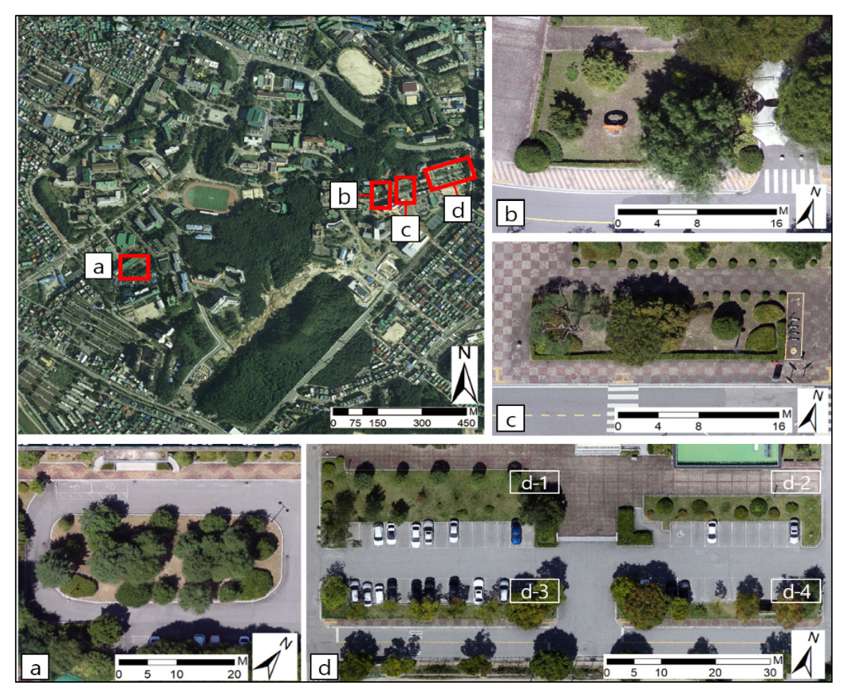
In this study, time-series ST changes were analyzed according to the components of UGSs targeting four green spaces (classified as a, b, c, and d) in Kangwon National University, Chuncheon, Gangwon-do, Korea (Fig. 1). The study sites selected were green spaces that were relatively less affected by the shadows of buildings and facilities, as they were located to the south centered on nearby buildings. In addition, they were surrounded by planting strips on all sides, and had varying vegetation statuses (conifers, deciduous trees, mixed forests) and vertical structures (tall trees, shrubs, multi-layer).
Study sites.
Green space (GS) “a” is in the shape of a rectangle with an area of about 611 m2. A 4-story concrete building in the northwest and a parking lot in the southeast are located around the GS, surrounded by an artificial surface, asphalt pavement. Tall trees and shrubs are planted in multiple layers in the GS, where Pinus densiflora, Pinus strobus, Taxus cuspidata, and Rhododendron yedoense are mainly distributed among the vegetation. GS “b” is in the shape of a trapezoid with an area of about 314 m2. A four-story concrete building and neighboring vegetation are located on the north side of the GS, surrounded by concrete sidewalk blocks and asphalt pavement. Trees and shrubs are planted in a single layer inside the green space, as well as a metal sculpture. The vegetation includes Acer palmatum, Quercus rubra, Magnolia denudata, Ginkgo biloba, Juniperus chinensis, Juniperus chinensis var. sargentii, Chaenomeles speciosa, Rhododendron yedoense, and Buxus koreana. GS “c” is in the shape of a rectangle with an area of about 182 m2. A 4-story concrete building and neighboring vegetation are located on the north side of the GS, surrounded by concrete sidewalk blocks. Trees and shrubs are planted separately in the GS, where the vegetation includes Acer palmatum, Prunus serrulata, Pinus densiflora, Taxus cuspidata, and Rhododendron yedoense. In addition, the inside of the green space is partially mounded, featuring a ground elevation difference of up to approximately 30cm and a curved shape of the ground. GS “d”, with a total area of about 1,228 m2, is divided into four planting zones. 5-story and 6-story concrete buildings are located on the north and west sides of the entire GS d, respectively, with a parking lot between the 4 planting zones. The vegetation inside GS “d-1” includes Diospyros kaki, Zelkova serrata, Acer palmatum, Picea abies, Pinus rigida, Lagerstroemia indica, Betula platyphylla, Juniperus chinensis, Juniperus chinensis var. sargentii, Cercis chinensis, Rhododendron yedoense, and Buxus koreana. The vegetation inside GS “d-2” includes Cercis chinensis, Taxus cuspidata, and Rhododendron yedoense, while Zelkova serrata and Chionanthus retusus are distributed inside GS “d-3”. Zelkova serrata, Picea abies, and Prunus armeniaca are planted inside GS “d-4”. The GSs are surrounded by concrete sidewalk blocks and asphalt pavement. Table 1 summarizes the data on the area, spatial characteristics, and vegetation distribution of the study sites.

Status of area, spatial characteristics, and vegetation distribution of the study sites
Building data on UGSs
UAV filming and image processing
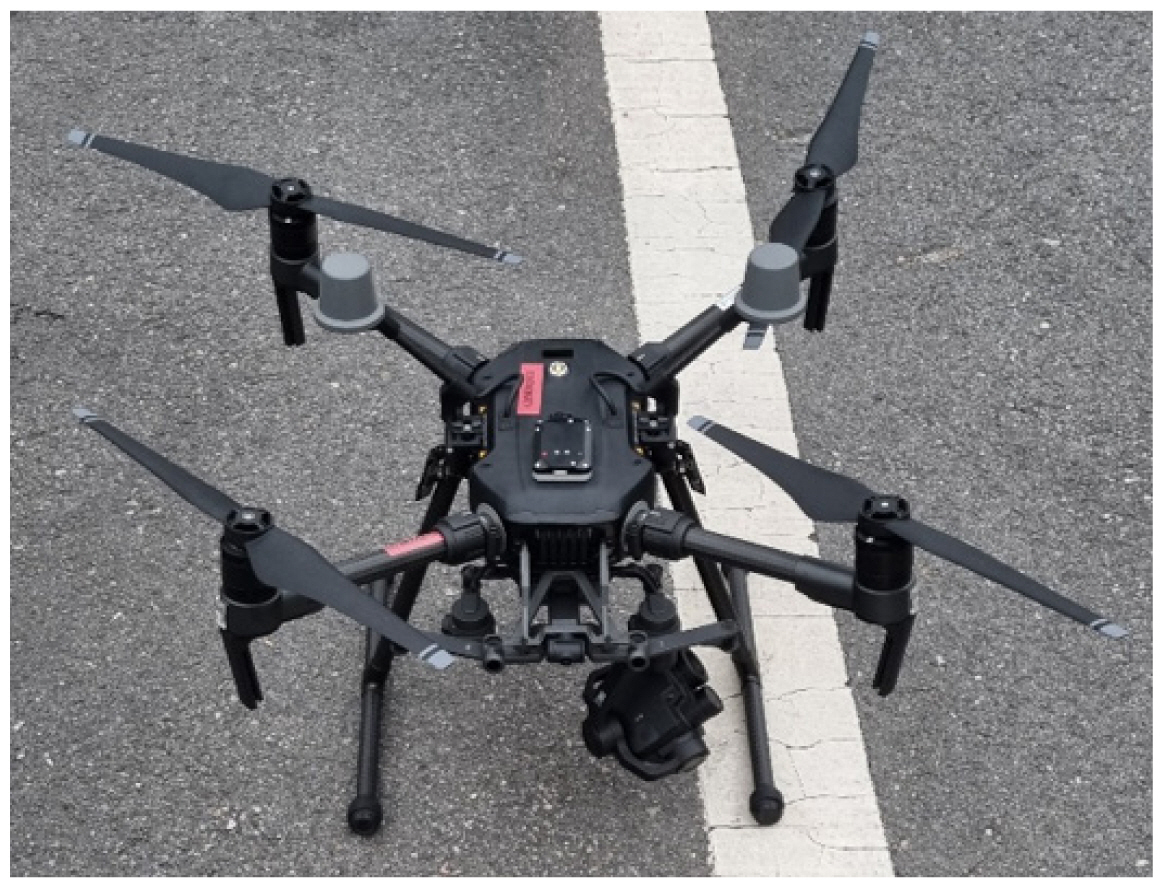
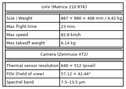
For UAV filming, DJI Matrice 210 RTK was used, which was equipped with high-precision Global Navigation Satellite System (GNSS) receiver cards and real-time kinematic (RTK) modules, enabling precise data acquisition without installing a separate ground control point (GCP) (Lee et al., 2021). In addition, the camera mounted on the UAV was a thermal imaging camera Zenmuse XT2, allowing us to obtain both thermal and RGB images. The specifications of the equipment are shown in Table 2.
Specifications of UAV and thermal camera
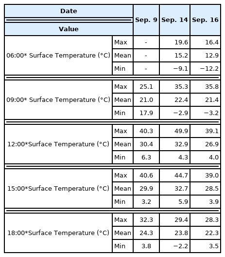
To acquire ST data of UGSs, UAV flight and filming were conducted on September 9, 14, and 16, 2021, by selecting days with few clouds and low wind. On the 9th, 14th, and 16th, the days of UAV filming in Chuncheon-si (the location of the study sites), the average temperature was 21.7, 23.2, and 21.5°C, respectively, and the average wind speed was 1.2, 2.7, and 1.7m/s, respectively (KMA) Weather Nuri, 2022).
UAV flight and filming were conducted at 09:00, 12:00, 15:00, and 18:00, which were three-hour intervals based on 06:00, the time when the ground surface was not exposed to solar heat. Considering the max flight time of the equipment and the distance between the study sites, two flights were conducted at each time point, totaling 30 flights a day. Pix4d Capture software provided by DJI was used for the UAV flight and filming; after setting the altitude to 70 m, overlap to 90%, and flight speed to 5 m/s, the pictures were taken with the automatic flight function. First, GAs b, c, and d were taken, and after equipment inspection and battery replacement, a relatively distant GS a was taken (Fig. 2 ). For each flight session, efforts were made to complete the shooting within 1 hour.
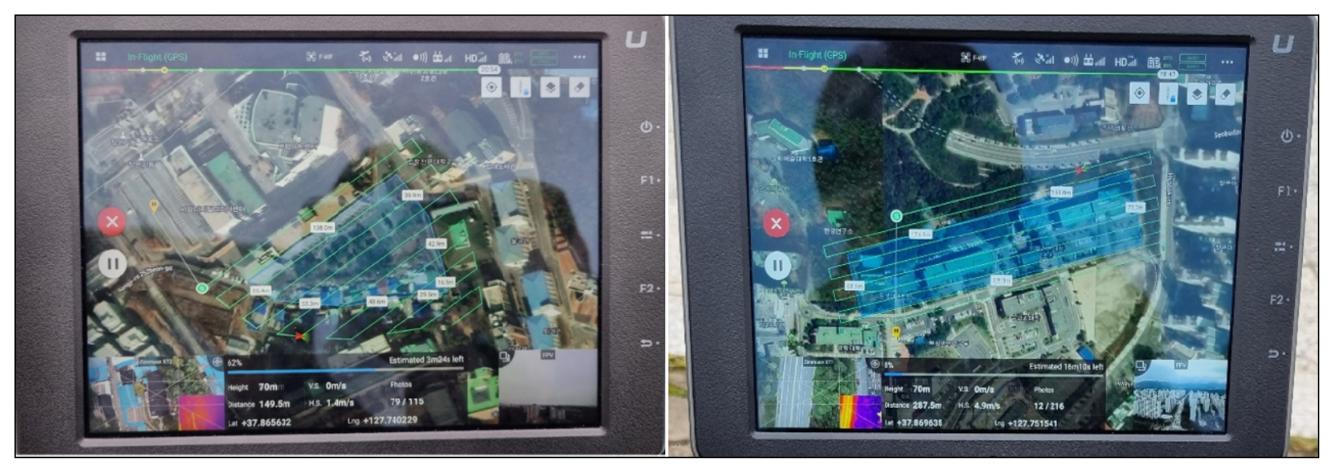
UAV controller screen capture (Left: Filming route for GS a; Right: Filming route for GSs b, c, and d).
The images acquired from the UAV were processed into thermal orthoimages (“ST orthoimages” hereinafter) using Pix4Dmapper, which is software capable of producing orthoimages. RGB orthoimages were produced for each study site using RGB images acquired at 12:00 on September 14th. WGS84/UTM zone 52N was used as an orthoimage coordinates system. In addition, all ST and RGB orthoimages produced were adjusted to the same spatial location for each GS using the georeferencing tools of ArcGIS software (v10.3.1). Then, using the Extract by Mask tool, the ST and RGB orthoimages of the study sites were generated. A total of 57 ST orthoimage data were constructed by excluding filmed images for which ST orthoimages were not generated due to an error in the Pix4Dmapper software: 06:00 flight sessions Sep. 9 for GSs a and b; and 12:00 session Sep. 16 for GS c.
Determining the status of UGSs and measuring the ST
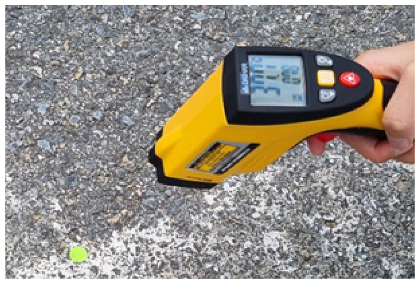
To grasp the status of each GS and analyze the accuracy of the ST data obtained from the UAV, a field survey of ST was conducted. The status of each GS was surveyed to grasp the location of trees and facilities on September 13, 2021. In addition, the ST was measured using DH. The3017 (DAIHAN), a portable infrared thermometer (Table 3). Eight ST measurement points were selected, and each time the UAV passed over the points, the ST was measured three times and averaged (Fig. 3). Considering the surface material characteristics of measurement points, the emissivity of the equipment was set to 0.92 for green areas (grass), 0.85 for sidewalk blocks (red bricks), 0.95 for asphalt pavements, and 0.95 for metal sculptures (Jeong, 2009).
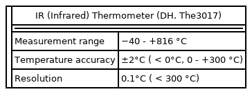
Thermometer specification
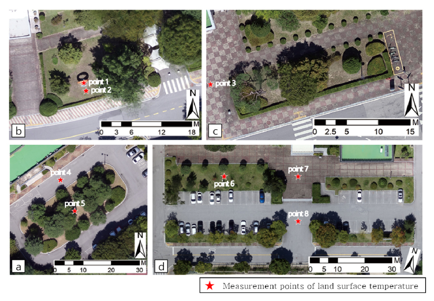
ST measurement points using an infrared thermometer.
ST change analysis of UGS components
An analysis of ST changes in UGS components was conducted based on ST orthoimages and field survey data constructed by filming at 06:00, 09:00, 12:00, 15:00, and 18:00 on September 9, 14, and 16. The components of UGSs were classified into coniferous and deciduous trees, shrubs, grass, metal sculptures, and paved roads according to tree characteristics, land-cover materials, and facilities. First, the accuracy of the data acquired by the UAV was verified by comparing the values measured through the portable ST measuring device with those of the ST orthoimages. To verify accuracy, an independent sample t-test was performed using IBM SPSS Statistics (ver. 24).
In addition, by comparing the RGB orthoimages generated with the status data of the GSs (location of trees and facilities) acquired through the field survey, the GSs were mapped to classify land cover types within the areas using ArcGIS (v10.3.1) software. Then, to extract ST values, random points were generated for ST orthoimages for each GS. Based on one random point per 1 m2 of GS area, 611 points were generated for GS a, 314 for GS b, 182 for GS c, and 1,228 for GS d. After this, the UGS components and ST values of the generated points were extracted using the Extract Multi Values to Points tool.
Finally, to analyze the change in ST according to UGS components, a one-way ANOVA was conducted to compare the average ST values for each UGS component. Since the result of Levene’s test did not meet the assumption of homogeneity of variance (p = .003), a Welch’s ANOVA was performed. Mean differences in each UGS component were analyzed through Dunnett’s T3 post-hoc test (used when the assumption of equal variance is not met).
Results and Discussion
ST orthoimages of UGSs
For an analysis of time-series ST changes in UGSs, ST orthoimages and green-space type maps of the study areas were generated, which were based on images acquired by UAV filming and field survey at 06:00, 09:00, 12:00, 15:00, and 18:00 on September 9, 14, and 16, 2021.
GS a (multi-layer planting of trees/shrubs)
Fig. 4 and Table 4 show the ST orthoimages and green-space type maps of GS a generated for each flight session. As the altitude of the sun increased based on 06:00 session, the distribution change of the average ST in GS a in each flight session had a tendency to increase by 16.0°C for 12:00 session, reach peak ST in the 12:00 and 15:00 sessions, and decrease by 6.9°C in the 18:00 session. The daily maximum ST was found in asphalt pavement and grass, and the daily minimum ST was found in streetlights. For asphalt pavements, as the average heat storage in summer is 511.2 W/m2, which is higher than that of other natural surface materials (455.7 W/m2 for grass, 463.3 W/m2 for wood), they seem to have the highest ST (Jo and Wu, 2015). In addition, the ST of grass varies depending on the degree of soil exposure, but it can be higher than that of artificial surface materials including roads and buildings (Zhao et al., 2017). Bare soils located in cities seems to have high ST due to their low soil moisture content (Sayão et al., 2020). On the other hand, it seems that streetlights had a relatively low ST, since they consist of a metal material with high solar reflectance and have a heat dissipation function inside that emits heat to the outside (Oh, 2009).

ST orthoimages and green-space type map of GS a.
Maximum, average, and minimum ST values extracted from ST orthoimages of GS a
The average ST increase in GS a was 16.0°C, which was the smallest when compared to that in GS b (16.4°C), GS c (19.9°C), and GS d (18.9°C); it appears that the ST increase was relatively small due to the functions of trees such as evapotranspiration and solar radiation absorption (Jo and Ahn, 1999). In particular, for GS a, where the trees are multi-layered and densely planted with many crowns overlapped, compared to GSs b, c, and d, it is considered that this may have been the result of a greater effect of tree functions.
GS b (Single-layer planting of trees/shrubs)
Fig. 5 and Table 5 show the ST orthoimages and green-space type maps of GS b generated for each UAV flight session. As the altitude of the sun increased based on the 06:00 session, the distribution change of the average ST in GS b for each flight session tended to increase by 16.4°C for the 12:00 session, reach the highest ST for the 09:00 and 12:00 sessions, and decrease by 6.7°C for the 18:00 session. The daily maximum ST was found in cars stopped around the planting zone and metal sculptures inside the GS, and the daily minimum ST was found in streetlights. For cars and metal sculptures, which consist of metal materials with high thermal conductivity, it seems that high STs were caused by continuous solar radiation at midday (Kim et al. 2020). The streetlights were the same as in GS a above.
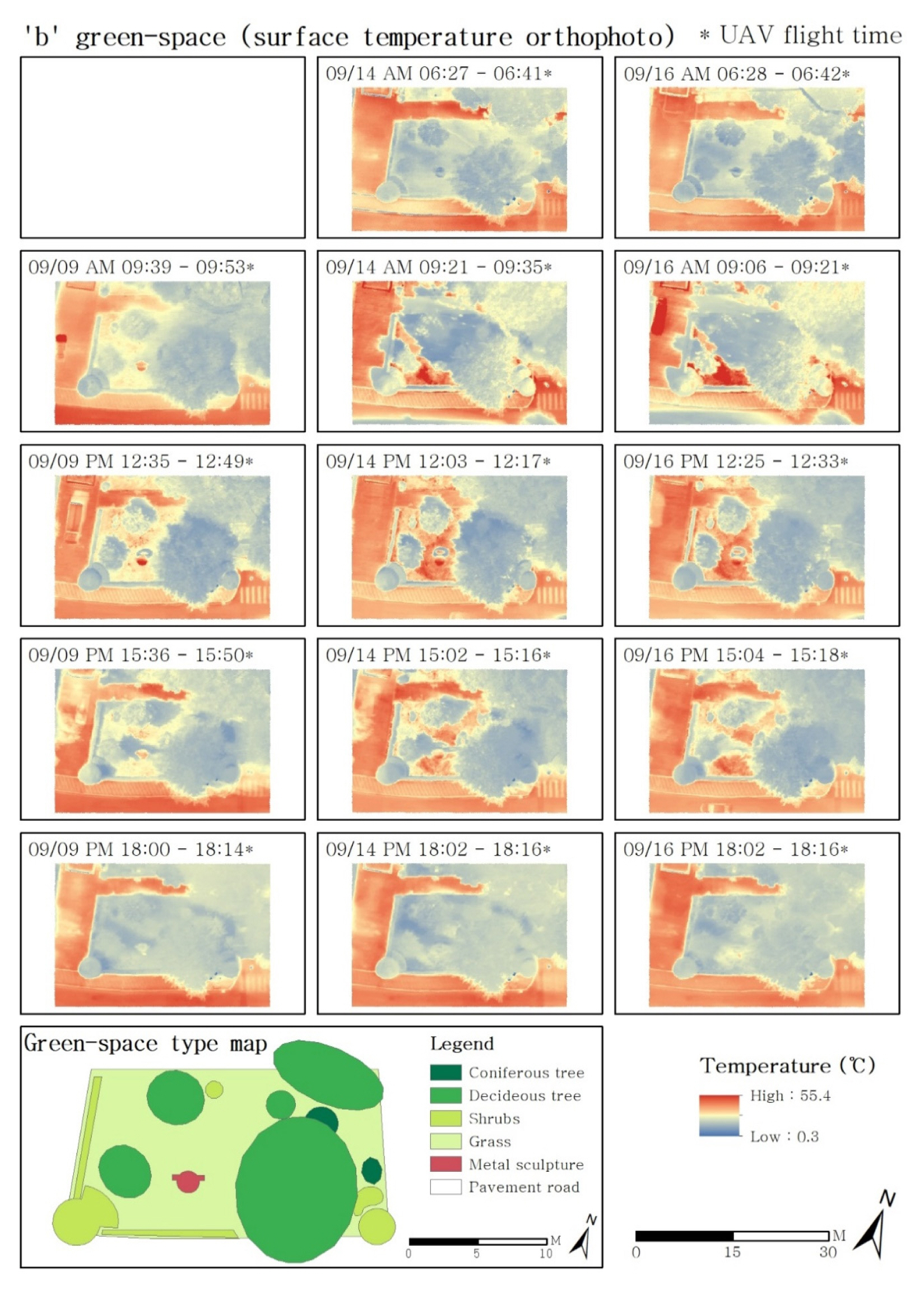
ST orthoimages and green-space type maps of GS b.

Maximum, average, and minimum ST values extracted from ST orthoimages of GS b
The average ST rise of GS b was found to be 16.4°C, 0.4°C higher than that of GS a (multilayer planting of trees/shrubs) and 2.9°C lower than that of GS c (separate planting of trees/shrubs). Based on this, in terms of ST improvement in urban summer, it is confirmed that dense planting of trees is more effective than individual planting, and multi-layer planting is more effective than single-layer planting. In addition, it is found that the degree of soil exposure inside the GS has a significant effect on the ST rise at midday.
GS c (separate planting of trees and shrubs)
Fig. 6 and Table 6 show the ST orthoimages and green-space type maps of GS c created for each session. As the altitude of the sun increased based on the 06:00 session, the change in distribution of average ST by session in GS c tended towards increasing by 19.9°C for the 12:00 session, reaching the highest ST for the 09:00 and 12:00 sessions, and decreasing by 9.6°C at 18:00. The daily maximum ST was found in the grass, and the daily minimum ST was found in the streetlights. Notably, for the grass inside GS c, as the degree of soil exposure was partially severe compared to GSs a, b, and d, and the soil moisture content was lowered by exposure to solar radiation for a long period of time in summer, it seems that the ST at midday was high (Sayão et al., 2020). The streetlights were the same as in GS a above.
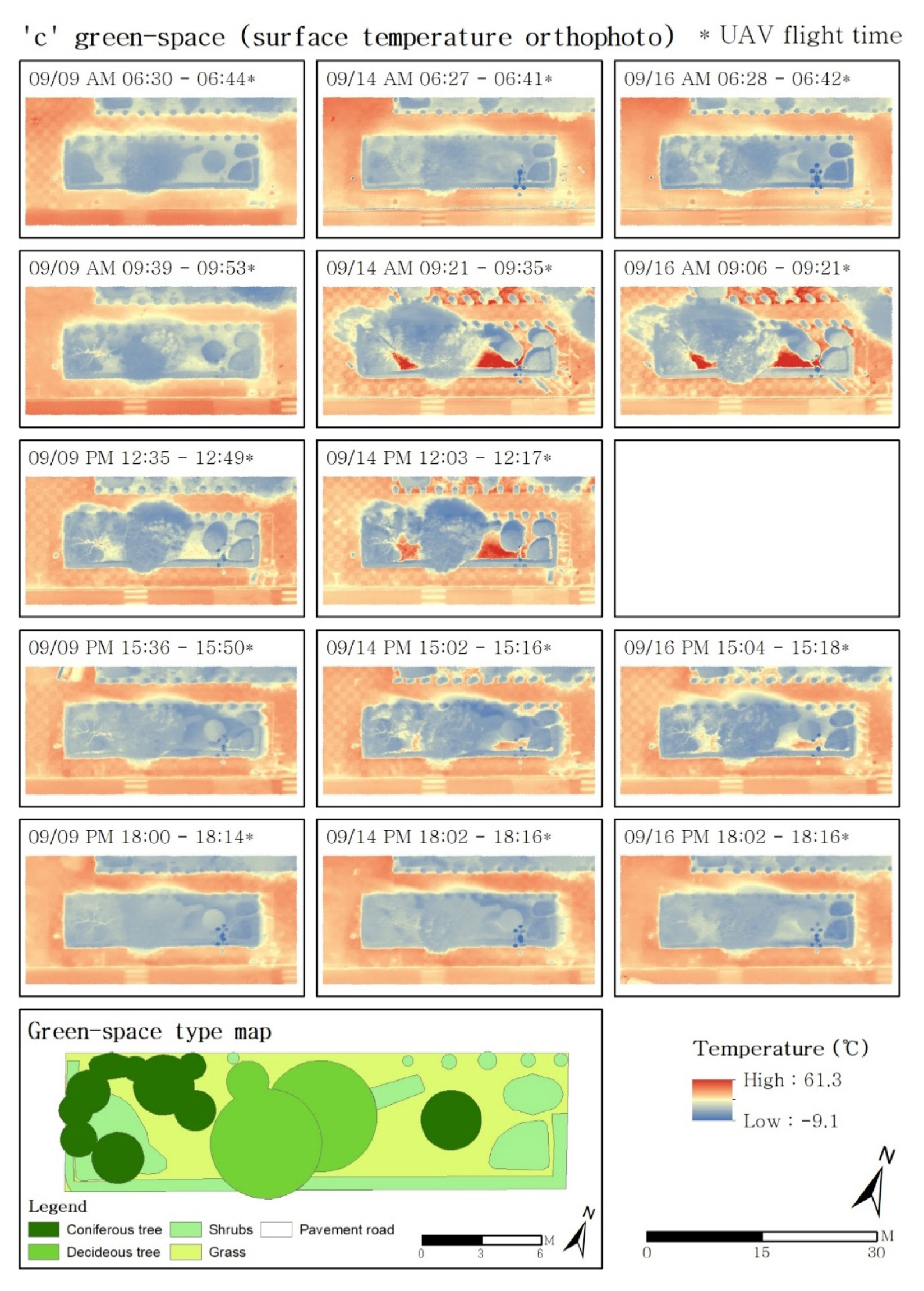
ST orthoimages and green-space type maps of GS c.
Maximum, average, and minimum ST values extracted from ST orthoimages of GS c
The average ST rise of GS c was found to be 19.9°C, which was the largest of all the GSs. The main cause of the rapid increase in ST at midday is considered to be the severely bare soil inside the GS, as described above. In addition, it seems to be caused by a combination of several factors, including mounds within the GS, and the limited shadow generation due to the separate planting of trees and shrubs.
GS d (planting around the parking lot)
The ST orthoimages and green-space type maps of GS d generated in each session are presented in Fig. 7 and Table 7. As the sun’s altitude increased based on the 06:00 session, the distribution change in average ST of GS d by session tended to increase by 18.9°C for the 12:00 session, reaching a peak, and to decrease by 9.2°C for the 18:00 session. The daily maximum ST was found in cars parked in the parking lot, and the daily minimum ST was found in the streetlights. As described above, for cars made of metal materials with high thermal conductivity, it seems that high STs were caused by continuous solar radiation at midday (Kim et al. 2020). For streetlights, it seems that low STs were caused by high solar reflectance, and a heat dissipation function formed inside (Oh, 2009).
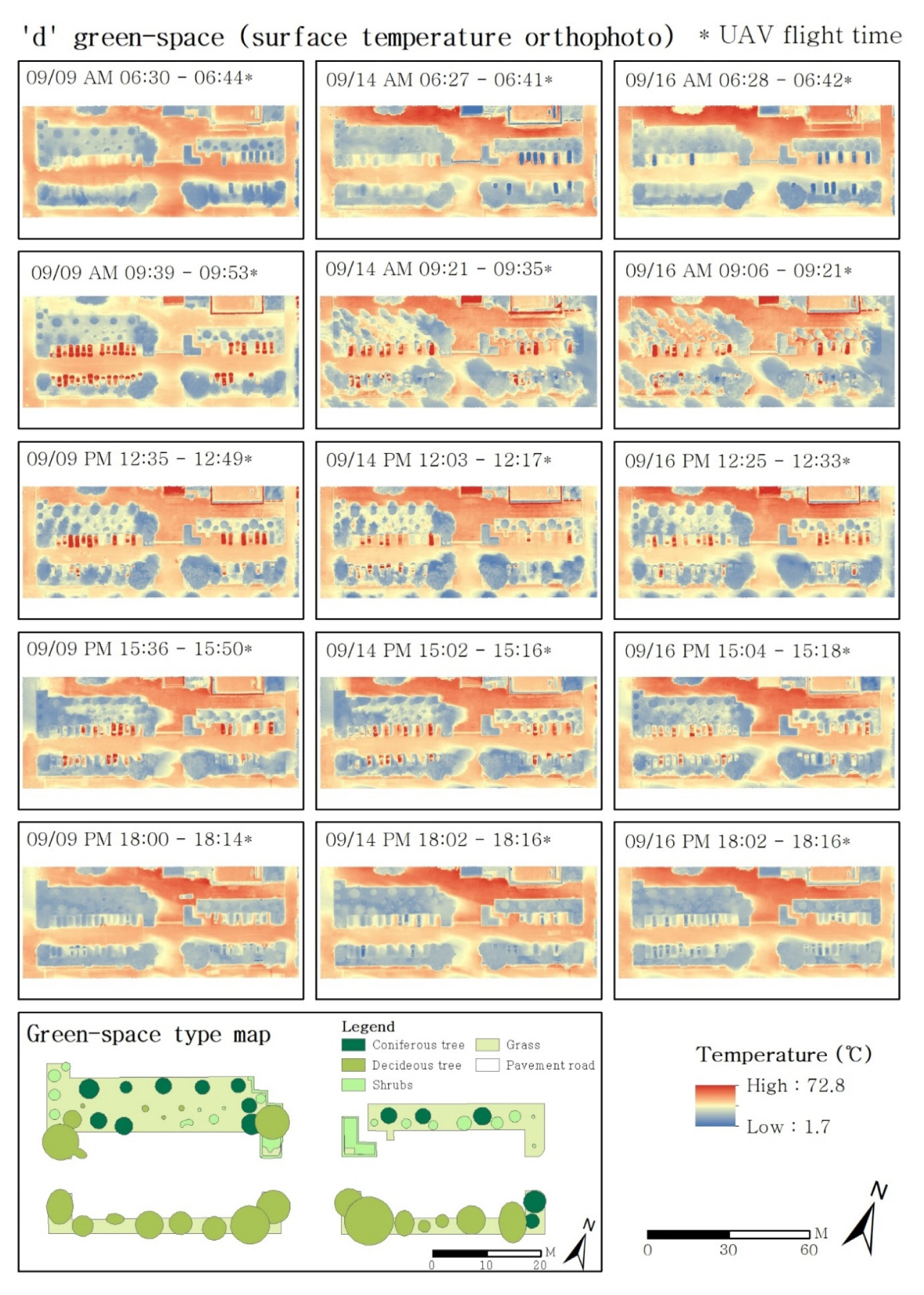
ST orthoimages and green-space type maps of GS d.
Maximum, average, and minimum ST values extracted from ST orthoimages of GS d
The average ST rise of GS d was 18.9°C, which was found to be 2.5°C higher than that of GS b (single-layer planting of trees/shrubs) with a similar planting type. This seems to be the result of differences in spatial characteristics around the GSs; the number of parked cars and the neighboring land cover (e.g., material properties, area) may have a significant impact on ST variability (Naughton and MacDonald, 2019). In particular, the amount of sensible heat that moves from the top of cars into the atmosphere at midday can have a significant effect on the rise in ambient temperature. Ahn et al. (2007) reported that such amount from parked cars was estimated to be about 60 W/m2 higher than that of hot asphalt pavements.
Accuracy verification of ST orthoimages
To verify the accuracy of the generated ST orthoimages, an independent sample t-test was conducted on the ST values extracted from the orthoimages and those actually surveyed using a portable infrared thermometer (115 samples). The resulting t-value was 0.150, with a p-value of 0.881 ( > .05), which was not statistically significant (Table 8). That is, it was found there was almost no average difference between the values calculated from the ST orthoimages (28.76°C), and those actually surveyed (28.94°C). It was confirmed that the temperature values from the generated ST orthoimages had high accuracy even in comparison with those actually measured.

T-test results for temperature values from ST orthoimages and those actually measured
ST change analysis of UGS components
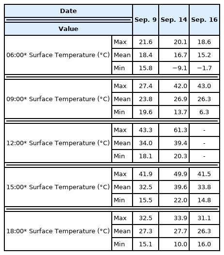
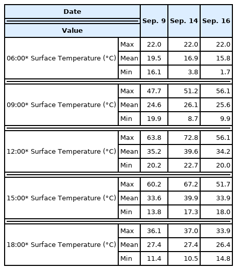
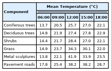
Based on the results of the analysis of the ST distribution of UGS components (conifers, deciduous trees, shrubs, grass, metal sculptures, pavement) according to the UAV flight session (06:00, 09:00, 12:00, 15:00, and 18:00; Fig. 8; Table 9), for the 06:00 session, conifers (13.7°C) had the lowest average ST, followed by metal sculptures (13.8°C), shrubs (14.4°C), deciduous trees (14.8°C), grass (14.9°C), and pavement (17.8°C). For the 09:00 session, the average ST of conifers (20.6°C) was the lowest, followed by shrubs (21.7°C), deciduous trees (21.9°C), metal sculptures (22.1°C), grass (23.7°C), and pavement (25.4°C). For the 12:00 session, the average ST of conifers was the lowest (25.7°C), followed by deciduous trees (27.38°C), shrubs (28.4°C), grass (34.3°C), pavement (38.2°C), and metal sculptures (41. 9°C). For the 15:00 session, the average ST of conifers and shrubs (27.0°C) was the lowest, followed by deciduous trees (27.8°C), grass (30.1°C), metal sculptures (33.9°C), and pavement (38.2°C). Finally, for the 18:00 session, average ST was the lowest for grass (22.0°C), followed by conifers (22.1°C), shrubs (22.1°C), deciduous trees (22.9°C), metal sculptures (23.5°C), and pavement (28.7°C).

ST distribution of UGS components.
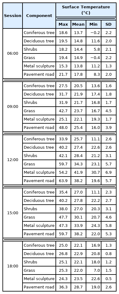
ST values of UGS components
By performing an analysis of variance (Welch’s ANOVA) to compare the ST mean values of the UGS components (Table 10), the significance probability (p-value) of the F-value for all sessions was found to be 0.000, indicating that the difference in ST between the UGS components was statistically significant. A post-hoc test of the 12:00 session with the highest TS values found that there were significant differences between conifers (25.7°C) and the other five components, including deciduous trees (27.4°C), shrubs (28.4°C), grass (34.3°C), metal sculptures (41.9°C), and pavement (38.2°C); ST differences between them were 1.7°C, 2.7°C, 8.6°C, 16.2°C, and 12.5°C, respectively, showing that the mean value of conifers was the lowest. Deciduous trees (27.4°C) showed significant differences from shrubs (28.4°C), grass (34.3°C), metal sculptures (41.9°C), and pavement (38.2°C); ST differences were 1.0°C, 6.9°C, 14. 5°C, and 10.8°C, respectively, indicating that the mean value of deciduous trees was the lowest. Shrubs (28.4°C) showed significant differences from grass (34.3°C), metal sculptures (41.9°C), and pavement (38.2°C); ST differences were 5.9°C, 13.5°C, and 9.8°C, respectively, showing the lowest mean value of shrubs. Finally, grass (34.3°C) showed significant differences from metal sculptures (41.9°C) and pavement (38.2°C); the ST differences were 7.6°C and 3.9°C, respectively, indicating the lowest mean value of grass.
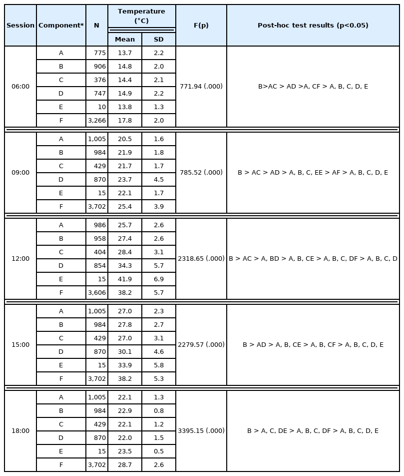
Results of Welch’s ANOVA for ST differences depending on UGS components
Based on the post-hoc test results of all sessions, conifers, deciduous trees, shrubs, and grass, which are vegetation, had lower STs than pavement. Compared to pavement, the ST was 4.1–12.5°C lower for conifers, 3.0–10.8°C for deciduous trees, 3.4–11.2°C for shrubs, and 1.7–8.1°C for grass. For the 12:00 session, where the effect of shadow was relatively small, the ST difference between pavement and vegetation was the largest in conifers (12.5°C), followed by deciduous trees (10.8°C), shrubs (9.8°C), and grass (3.9°C). Although previous studies reported that the ST of broad-leaved trees is lower than that of conifers in forests (Arx et al., 2012; Kim, 2004), Choi et al. (2017) found that in landscape planting sites, conifers can have a lower ST than broad-leaved trees depending on the tree condition and surrounding environment. In addition, compared to other components, grass and pavements were found to exhibit a wide range of ST. This seems to be attributed to shadows created by neighboring buildings, vegetation, and cars (e.g., parking lots) as the sun’s altitude changes; that is, the parts exposed to solar radiation have high STs, while the shadowed parts have low STs (Naughton and MacDonald, 2019).
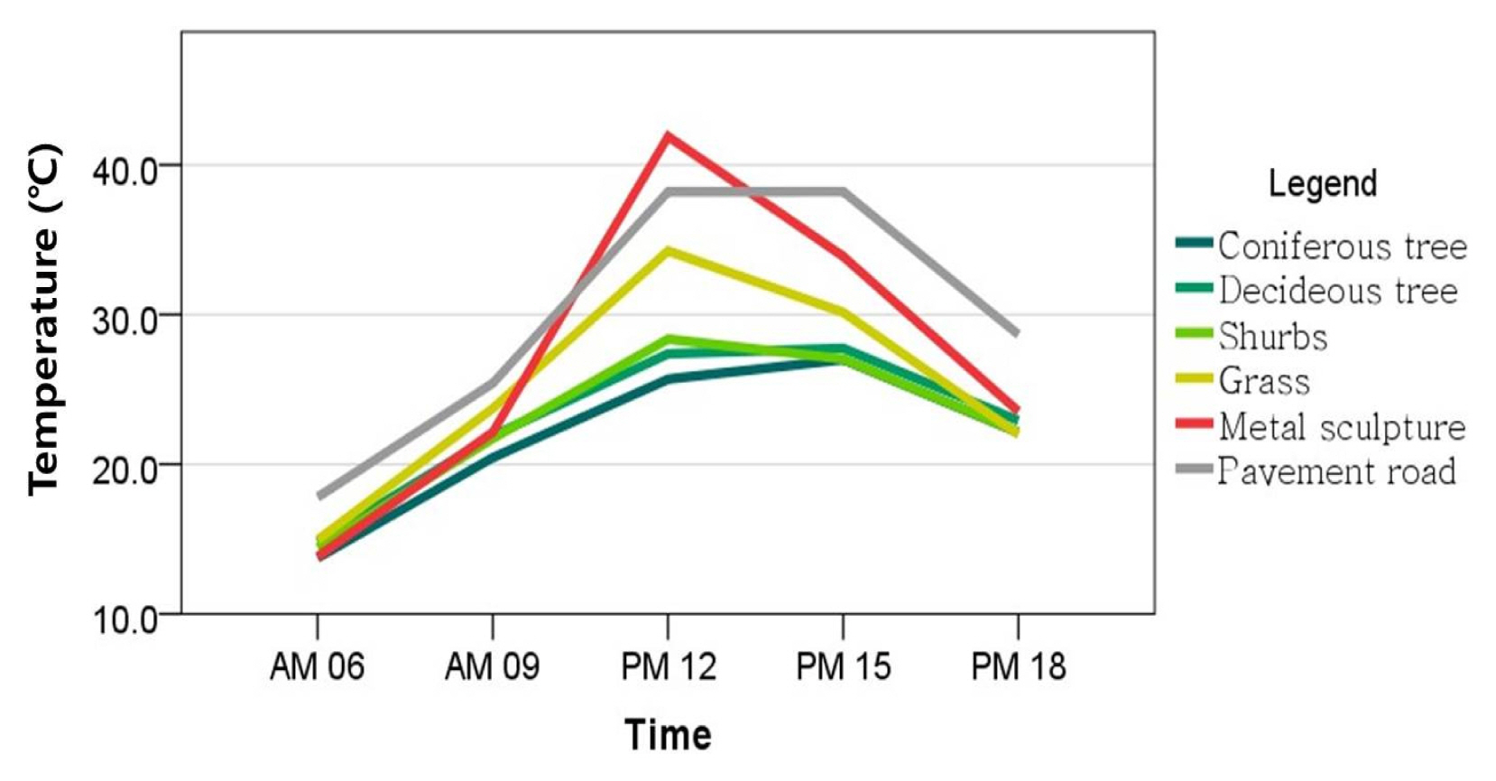
Finally, by comparing changes in mean ST of UGS components over time (Fig. 9; Table 11), it was found that the time-series ST change of metal sculptures (28.1°C) was the largest, followed by pavement (20.4°C), grass (19.4°C), shrubs (14.0°C), conifers (13.3°C), and deciduous trees (13.0°C). Since the ST of metal sculptures with high thermal conductivity reacts sensitively to the surrounding environment (Kim et al., 2020), it seems that their ST rapidly changed around 12:00 pm depending on whether the solar radiation reached the surface. Pavements with low albedo for solar radiation feature high average heat storage and heat absorption in summer (Jo and Wu, 2015), and the ST increased rapidly for 12:00 session due to solar radiation at midday. In addition, the ST for the 06:00 and 18:00 sessions, when solar radiation is relatively low, was 2.9–6. 7°C higher than other components, which seems to be attributed to the thermal effect due to the characteristics of heat storage. On the other hand, conifers, deciduous trees, shrubs, and grass exhibited smaller ST changes than artificial materials including metal sculptures and pavement; it seems that the functions of trees and soil, including evapotranspiration and absorption of solar radiation, enabled them to have relatively low STs even under solar radiation at midday (Jo and Ahn, 1999). For grass, the variation in ST was 5.4 to 6.4°C larger than that of conifers, deciduous trees, and shrubs, which seems to result from the fact that the degree of heat release of grass is greater than that of tree crowns (Feng et al., 2020).
Changes in mean ST of UGSs.
Mean STs of UGSs
Integrating the above results, it was found that the STs vary depending on characteristics such as the difference in solar radiation over time, the albedo of UGS components, and thermal conductivity. In addition, as UGSs showed a relatively lower ST than artificial surfaces, it is considered to be more effective to use natural elements than artificial ones to improve the urban thermal environment.
Conclusion
In this study, in terms of improving the thermal environment of urban areas in summer, the ST and spatial characteristics of UGSs were determined, and the time-series changes in ST depending on spatial characteristics were analyzed. To this end, data on STs and components (conifers, deciduous trees, shrubs, grass, metal sculptures, pavements) of UGSs at 06:00, 09:00, 12:00, 15:00, and 18:00 were constructed through UAV and field surveys.
Through analyzing the ST distribution depending on the UGS components, it was found that the ST of conifers, deciduous trees, shrubs, and grass, which are vegetation, was lower than that of paved roads: for conifers, 4.1–12.5°C lower than paved roads; for deciduous trees, 3.0–10.8°C lower; for shrubs 3.4–11.2°C lower; and for grass 1.7–8.1°C lower. For the 12:00 session, when the effect of shadow was relatively small, the ST difference between pavement and vegetation was the largest in conifers (12.5°C), followed by deciduous trees (10.8°C), shrubs (9.8°C), and grass (3.9°C). In addition, the variations in ST over time were greatest for metal sculptures (28.1°C), followed by pavement (20.4°C), grass (19.4°C), shrubs (14.0°C), conifers (13.3°C), and deciduous trees (13.0°C). Based on the results of this study, of the vegetation, conifers were the component with the lowest surface temperature, followed by deciduous trees, shrubs, and grass; deciduous trees were the component with the smallest variations in ST over time, followed by conifers, shrubs, and grass. As such, it was found to be necessary to consider the UGS components for the efficient planning and management of UGS in terms of improving urban thermal environment.
With rapid urbanization, UGS is gradually decreasing and becoming more fragmentated; there is also a limit to creating wide green spaces in cities that have already been developed at high density. Since it is relatively easy to develop green spaces in urban areas by replacing them with artificial surfaces, the urban heat environment in summer has been getting worse. In addition, in South Korea, excessive pruning is performed on some roadside trees for reasons that include tree crowns covering signboards in shopping malls, contact with power lines, and sidewalk width restrictions, which in turn, gradually degrades the function of UGSs. Therefore, it was considered necessary to quantitatively analyze the relationship between the benefits provided by UGSs and spatial characteristics. This study aimed to suggest the need for the planning, creation, and management of UGSs, focusing on the aspect of improving the urban thermal environment.
As study sites, this study targeted some areas of a university campus for the convenience of data construction, which may cause differences from the results of UGSs in other regions. For urban areas, buildings and paved roads are dominant compared to suburbs or rural areas; the dense population and the relatively large amount of heat accumulated can further exacerbate urban thermal environment. In addition, the urban thermal environment can be changed by regional spatial characteristics (e.g., rivers) and detailed spatial characteristics (e.g., land use status) (Jo and Ahn, 2009; Oh and Hong, 2005; Park et al., 2016). However, in this study, it was found that UGSs exhibited relatively lower STs than artificial surfaces; thus, using natural rather than artificial materials was more effective in improving the urban thermal environment.
Finally, when acquiring data using UAVs, there is a limitation in that some data could not be acquired within the planned time due to problems that included delays in equipment preparation and travel time, equipment defects, and on-site conditions to be considered. In addition, since the urban thermal environment can be affected by a combination of factors, including the locations of surrounding buildings and roads, direction and speed of wind, size of green spaces, and species and arrangement of trees, it is necessary to add them to the components and evaluate them comprehensively. As such, future research should examine and evaluate various samples of UGSs and the additional factors influencing urban thermal environment. Through this, it is expected that specific measures for planning, creation, and management of UGSs can be presented in terms of thermal environment improvement.
Notes
This study utilized some of the data from Lee SB’s master’s thesis (2022). Also, this work was conducted with the support of the Korea Environment Industry and Technology Institute via the Urban Ecological Health Promotion Technology Development Project. It was funded by the Korea Ministry of Environment (grant no. 2019002760001).