Mapping the Mangrove Forest Restoration Potential and Conservation Gaps in China Based on Random Forest Model

Study area

The study area is located between latitude 18°12′-27°32' N and longitude 108°03′-120°22' E across 2,510,934.2 ha coastal areas. Since 1990, 30 mangrove nature reserves have been constructed in the study area, including seven national nature reserves (six internationally essential wetlands). The scope of the study area and current mangrove reserves are shown in Fig. 2.

Fig. 2

Study area and mangrove occurrence locations and reserves. The study area included approximately 9,515 kilometers of mainland coastline (Guangxi, Guangdong, Fujian, Hong Kong, and Macau) and 3,001 kilometers of island coastline (Hainan, Taiwan), the northernmost city of Fuding, Fujian Province (27°32' N), and the southernmost city of Sanya, Hainan Province (18°12' N).

Occurrence dataset

Remote sensing imagery of the spatial distribution of mangroves in the study areas was obtained from National Earth System Science Data Center, National Science & Technology Infrastructure of China (http://www.geodata.cn) (2015, resolution 30 m) (Jia et al., 2019; Jia et al., 2018). We used field survey sample points and the google map (resolution 0.5 m) to evaluate the accuracy of the classification results and the overall mangrove forest. Optimized the mangrove distribution data (2015) and evaluated the classification results using landsat8 OLS remote sensing images. Displayed remote sensing images by false-color synthesis method (Yin et al., 2012) and overlayed the classification data. The classification accuracy was > 90%. These processes were performed in ArcGis10.5.

Field data survey

We gathered ground reference data to guide the model's training and analyze the final map's accuracy. The sampling plots were conducted along the coastline with a dimension of 30 m × 30 m. Also, the field data survey was conducted to identify the classification of mangrove types and their distribution circumstances.

Environment variables dataset

The mangroves' distribution is determined by biophysical and bioclimatic variables in the coast area. Based on the current database, we used four groups of environmental variables, including 19 climate factors, seven seawater factors, three topographic data, and ten soil data. Their meanings are shown in Table 1. and Fig. 4. All 39 environmental factors were regarded as ecological variables. (Guisan and Zimmermann, 2000; Shih, 2020).

Table 1

Environmental factors used for RFM

Fig. 4

Present condition of various aspects (Mean temperature of the wettest quarter, Mean temperature of the warmest quarter, Precipitation of the warmest quarter, Elevation, Bulk density, Coarse fragments, Mean sea surface temperature of the wettest quarter, and Mean sea surface of the warmest quarter).

The sampling process was as follows: (1) Identified the sampling data range (within the coastline extending 2 km inward and 1 km outward). (2) Divided the study areas into 1 km × 1 km raster data, it was believed that the environmental variables in each grid were consistent. (3) Cut and project the environmental variables into raster data and the mangrove raster data to form an occurrence dataset.

Soil parameters were retrieved from https://soilgrids.org/. Temperature and precipitation parameters were achieved from www.worldclim.com with a spatial resolution of 1 km² (30 arc-seconds). Topographic variables, including elevation, were derived from the ETOPO1 data of the global relief model from NOAA (https://www.ngdc.noaa.gov/mgg/global/global.html). The compound topographic index (CTI) was calculated as (Hu et al., 2020). The sea surface temperature (SST) data was derived from NASA MODIS-Aqua Level-3 (http://oceancolor.gsfc.nasa.gov). All 39 environmental variables were interpolated to the exact 1 km spatial resolution for subsequent model prediction; the total number of these grids was 41,182. (5) Sampling points were extracted in each grid (1 km × 1 km) if mangroves exist. The value of these sampling points was 1; on the contrary, it was 0. The number of these grids where mangroves exist was 2,991. ArcGIS 10.5 software extracted the environmental variable values corresponding to the mangroves' distribution points and background points.

Random forest modeling process

A random forest model (RFM) was established based on presence-only data to evaluate suitable mangrove habitats. Random forest is a machine learning algorithm based on an ensemble learning theory developed by Breiman in 2001 (Breiman, 2001; Evans et al., 2011; Jordan and Mitchell, 2015; Mazumder et al., 2010). The Random Forest classification prediction accuracy assessment is based on out-of-bag (OOB) data. The mean decrease of Gini can assess the significance of predictors. We imported the Random forest and Raster packages into the R Studio 4.0.4. We took the environmental variable raster data as an input dataset, thereby acquiring the probability of mangrove suitability and the importance of the variables.

Furthermore, we used the real presence points of mangrove samples to analyze the habitat suitability and drew the environmental response curves of each essential variable. The predicted probability of 50% was used as the threshold to obtain a suitable interval for each variable. We used the Seaborn package in Python 3.7 edition to map the environmental response curve. The modeling process is shown in Fig. 3.

Fig. 3

The Random Forest modeling processs.

Model validation

For RFM, it is reliable to test its performance using the area Under the Curve (AUC) statistics of the Receiver Operator Characteristic (ROC) plot (Bradter et al., 2013; Evans et al., 2011). The AUC of the ROC plot is equivalent to the probability that a test record is correctly differentiated from a random point in the predefined background study area.

Based on the model's outputs, the grids with an occurrence probability of more than 50% were selected as suitable areas (Lopatin et al., 2016). Then, suitable habitat area was calculated in ArcGIS 10.5. The predicted result of RFM probability ranged from 0 to 1 in accordance with the pixel value of each grid. The mangrove suitable area was divided into three groups: suitable high zone ( > 0.7), suitable medium zone (0.5–0.7), the suitable low area (0.1–0.5).

Restoration potential estimation

RFM aims to map the potential restoration locations for mangroves in the study area according to the predicted probability of habitat suitability. Remote sensing images and field data surveys showed that some areas used to be wetlands or marshes. They were transferred into artificial coasts for urban construction and can hardly be transferred to mangroves permanently. In mapping the accurate areas that can be used for mangrove restoration, it is necessary to combine the predicted areas obtained from RFM with land use and land cover parameters (Ficetola et al., 2014; Vessella and Schirone, 2013).

Land use and land cover (LULC) data were derived from Globaland 30 (http://www.globallandcover.com). We introduced the reciprocal of land use and land cover index as a transfer coefficient to revise the restoration potential probability (RPP) (Zhuang and Liu, 1997). The transfer coefficient was assigned to each grid based on the 2020 LULC data of China with a 1-km resolution. (Table 2).

Table 2

The land use and land cover degree index and transfer coefficient

Mapping the potential restoration areas and conservation gaps

We obtained the distribution map of mangrove suitable habitat areas according to the RPP index. Also, we identified suitable habitat areas with medium and high probability as potential areas for mangrove restoration. The calculated restoration potential area is needed to subtract the area of existing mangrove forests reserves. Finally, the existing mangrove reserves and the map of the mangrove's potential suitable habitat areas were superimposed to recognize the conservation gaps of the mangrove forests. The conservation gap was defined as the sampling sites with a medium and high probability for restoration and less than 20% of existing mangroves under protection in each grid cell (1 × 1 km) (Sabatini et al., 2020).

Performance of the model and the environmental predictors

The AUC value showed that the training accuracy of the RFM performance reached 0.89, and the testing accuracy reached 0.91, indicating that the model results were highly reliable (Fig. 5). The mean decrease Gini illustrated the air temperature, sea surface temperature, precipitation, and topography had a significant contribution to the habitat suitability of mangroves (Fig. 6). In the RFM, response curves can be created to show how predicted probability occurrence depended on the value of each environmental factor. Eight sensitive variables from the different environmental factors were selected to lead the response curves (Fig. 7). Most curves had a single peak shape, displaying that the mangrove niche was relatively concentrated. The variable intervals with the probability of occurrence threshold of ≥ 50% were taken as the best distribution range (Table 3).

Fig. 5

ROC curves for prediction distribution of mangroves. Using the area under the curve (AUC) statistics of the receiver operating characteristic (ROC) plot to test RFM performance. The ROC plot is generated by plotting the false positive rate of a model prediction (1-specificity, here given as fractional predicted area) against the true positive rate (model sensitivity, given as 1-rate of false negatives). An AUC value between 0.9 and 1.0 indicates excellent model performance, 0.8–0.9 = good, 0.7–0.8 = average, 0.6–0.7 = poor, and 0.5–0.6 = insufficient.

Fig. 6

Mean decrease Gini. In the random forest model, percent contribution was calculated as the increase in regularized gain when using the variable in each iteration of the training algorithm. Permutation importance was calculated by the decrease in AUC when training with the permuted data. Mean decrease accuracy was used to evaluate the importance of factors, indicated the degree of decrease in prediction accuracy. The larger the value, the greater the importance of the variable.

Fig. 7

Response curves of eight important environmental factors influencing mangrove distribution (the blue points illustrate the real presence grids of mangroves).

Table 3

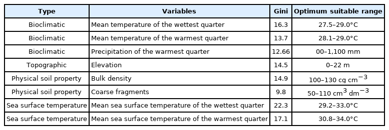
Variables with the top eight Gini index were regarded as major suitable factors

Field data survey

The field survey collected in situ exhibited that the mangrove forests in five coastal regions are divided into three types: Kandelia candel-Aegiceras corniculatum-Avicennia marina, Rhizophora stylosa-Bruguiera gymnorrhiza and Rhizophora apiculata-Xylocarpus granatum. Among the three types of mangrove forests, Rhizophora stylosa-Bruguiera gymnorrhiza (37.2%) and Rhizophora apiculata-Xylocarpus granatum (5.2%) were relatively less distributed, but mostly (90% of the total) were protected. Kandelia candel-Aegiceras corniculatum-Avicennia marina (71.6%) were mostly distributed and 52.6% protected.

Mangrove potential suitable habitat area and conservation gaps

The total theoretical area of mangroves' suitable habitat throughout the country was 196,566.6 ha. Here we have analyzed mangrove habitat geographical distribution characteristics from regions, latitudes, climate zones, and elevations. And we further investigated the conservation gaps in these regions.

In terms of mangrove suitable habitat distribution among regions, the predicted probability distribution of mangrove habitat suitability suggested that the medium and high suitable areas concentrated along the coastline in Guangdong, Guangxi, and Hainan provinces (Fig. 8). The predicted proportions of mangroves suitable habitat distributed in the five regions (Guangdong, Guangxi, Hainan, Fujian, and Taiwan) were listed in Table 4. The suitable habitat for mangroves in Guangdong and Guangxi provinces was estimated to be 110,666.3 ha and 68,691.2 ha. Comparatively, the proportion of potentially suitable Area in Fujian and Taiwan was relatively low. Our results indicated that the highly suitable areas for mangrove forests in Guangdong province were mainly concentrated along Beibu Bay, Leizhou Peninsula-Yangjiang Coast, and the Pearl River Estuary-Daya Bay. For Guangxi province, the highly suitable habitats were mainly located in Beibu Gulf, including Zhenzhu Bay, Qinjiang Estuary, Qinzhou Bay, Beihai Port, Anpu Port. In Hainan province, the highly suitable habitats were located in Gaolong Bay-Qinglan Port, Dongzhai Port, Chengmai Bay, Mianiao Bay, and a part of Beibu Bay. In Taiwan, there were no high-level suitable areas for mangroves restoration. Regarding mangroves habitat distribution along the latitude gradients, 92% of mangroves' suitable habitat ranged from 18°22' N to 24°44' N.

Fig. 8

Probability distribution of mangrove habitat suitability.

Table 4

Sum of potential suitable areas for mangrove restoration in five regions

Regarding mangrove suitable habitat distribution within different climate zones, over 80% of the mangrove area was located in the warmest zone, followed by the wettest zone (50%). Therefore, 90% of the mangrove area was located in the warm and wet zones (Fig. 7 (a) to 6 (b)).

Regarding mangrove suitable habitat distribution along the elevation gradients, 90% of mangroves are located in the area with an average elevation of less than 4 m. However, the range of predicted probability of mangrove suitable habitat distribution narrowed to 2 m. The predicted suitability decreased rapidly with the elevation over 2 m (Fig. 7 (d)).

These area statistics in different climate zones and elevation/ latitude gradients were not adjusted using the area-adjusted accuracy. No specific confusion matrix was available for each climate zone and elevation/latitude gradient; however, it did show the general suitability distribution of mangroves in different geographical regions.

The area of mangroves in the national nature reserves is currently 12,465.6 ha, accounting for 61.4% of the total mangroves, and 38.6% of the mangroves are distributed outside the reserves' boundaries are not strictly protected. In Fujian and Hainan provinces, most existing mangroves were under protection. In Guangxi province, the proportion of protected mangroves is the lowest, accounting for only 39.5% of this region's total area of mangroves. In these regions, only five mangrove wetlands were listed in the List of wetlands of international importance. Due to the limitation of the minimum area of declared national mangrove reserves, most of China's internationally important mangrove reserves are large and medium-sized, lacking small-scale mangrove reserves. Our results indicated that in Guangdong province, the conservation gaps mainly appeared in Leizhou Bay, Yangjiang Port, Zhenhai Bay, Shantou city Coastlines. For Guangxi province, the conservation gaps were mainly apeared in Beibu Gulf, including Zhenzhu Bay, Qinjiang Estuary, Qinzhou Bay, Beihai Port, Anpu Port. In Hainan province, conservation gaps occurred along the northwest coastline (Fig. 9). As for Taiwan, the conservation gaps mainly appeared in Beigang River estuary.

Fig. 9

Mangrove potential habitat suitable areas and conservation gaps. The mangrove reserve ( = protected mangrove forests), and conservation gaps ( = mangroves in areas with medium and high probability for restoration and with less than 20% existing mangrove forests under protection in each 1 km grid).

We suggested 24 potential sites for mangroves restoration (Fig. 9). We selected nine example sites as restoration opportunities for the further restoration zoning plan (Fig. 10), the sites information was listed in Table 5. Here, we specifically explained one example site, GD-11, how the environmental factors influenced the mangrove forests suitability, and why we chose them as restoration site.

Fig. 10

Selected potential areas for mangrove conservation and restoration plan. (red areas were designed as conservation zone, green areas were buffer zone, and yellow areas were restoration zone).

Table 5

Information of the selected potential areas for mangrove conservation and restoration plan

Mangrove restoration zoning plan

The components of the restoration concept plan were designed to take advantage of the unique site conditions and location within the selected restoration sites. The restoration concept plan includes three key zones: (1) buffer zone: restoration and agriculture Complex, (2) restoration zone: internal mangrove and marsh, and (3) conservation zone: external mangrove and marsh. The fundamental drivers of successful ecological community assembly at the chosen region are the tidal flows and substrate elevation.

The adjacent areas between restoration areas and agriculture and aquacultural areas can be designed as a buffer zone. The ecological development of this zone will build upon the idle aquaculture ponds and establish a restoration and agriculture complex. Further development of the restoration and agriculture complex will be achieved in three primary ways: expanding the area devoted to this system, introducing additional plant species to diversify the brackish marsh, introducing additional sediment in selected locations to create more areas of appropriate elevation, and diversifying site topography. Therefore, in this zone, additional fill will be used to diversify the topography further and create further opportunities to develop mangroves and marsh.

The restoration zone occupied by the internal mudflat and salt marshes has excellent potential for mangrove restoration. If the existing surface elevations are too low and the tidal range are too great, not allow for vegetation establishment (Pfadenhauer and Grootjans, 1999). Therefore, what the planning proposes for this zone is a phased, gradual reintroduction of tidal flows to achieve additional sediment accumulates in these areas.

In the conservation zone, sometimes, the remaining mangrove forests are exposed to open water. This ecological zone will be created by building structures in the open water zone, adjacent to the reserve within the seawalls, to encourage rapid sediment deposition. At current sediment deposition rates, it may take several decades for bottom elevations to increase to a level that would allow natural vegetation colonization. However, by strategic placement of bioengineering structures such as brush boxes and, potentially, the creation of artificial reefs using rock, the rate of sediment deposition can be significantly speeded in selected areas (Ren et al., 2011). Once appropriate surface elevations are achieved, mangrove and marsh species are expected to colonize them naturally, from propagules derived from zones 1 and 2. Techniques pioneered in this zone would have great potential to be useful elsewhere in the other region to restore or create mangrove habitat.

Restoration application in GD-11 site

Based on RFM prediction results (habitat suitability), mangrove forests conservation gaps analysis, and field survey, we found that GD-11 (Nansha Coastal Wetland, 22°36'N and 113°35'E) with high restoration potential and a good match with LULC data 2020. The site was comprised of approximately 1800 ha in the southern portion of Wanqingsha island, Guangdong. A review of historical satellite images showed that the site was in a relatively shallow zone where considerable sediment deposition was occurring. The coastline was accreting rapidly along the southern boundary of the selected site. Past reclamation activities have significantly reduced intertidal mudflat area and mangroves (Fig. 11). Therefore, we recommended that the mangrove forest restoration area should extend to include the suitable and high suitable zones scattered over the southern and southeastern part of this area.

Fig. 11

Reclamation patterns of the site GD-11.

Regional climate factor set important limiting parameters for mangrove habitat suitability. These parameters determine whether a self-sustaining ecological mangroves community can be established in the area. The climate of this region is subtropical oceanic monsoon. The average temperature of the warmest quarter is 29 °C in July to September. The average annual rainfall is 16,356 mm, with the most precipitation occurring from April to October (wettest and warmest quarter). The multi-year average temperature of surface water is 23.5 °C. Water temperature varies according to four distinct seasons; Spring: 24–27 °C, Summer: 28–30 °C, Autumn: 27–28 °C and Winter: 17–18 °C. Five mangrove forests species were reported as planted: Bruguiera gymnorrhiza, Kandelia candel, Sonneratia caseolaris, Sonnerati. apetala, and Aegiceras corniculatum. Both Kandelia candel, and Aegiceras corniculatum were reported occurring spontaneously which could better response to the regional environment. Indeed, choosing species with better environmental suitability is a better option, we suggested transplant Sonnerntia ovata to this site to rebuilt the ecological restoration systems.

For the further restoration zoning plan, we proposed the following recommendations: first, we designed the areas reclaimed between 1988 and 2000 as the buffer zone because agricultural fields and aquacultural ponds occupy this area. Buffering agricultural and aquacultural activities from sensitive receptors is a sound land use planning practice. Secondly, designed the areas reclaimed between 2000 and 2010 as the conservation zone, because, in the northeastern corner of the site, small areas of mangrove forests (Kandelia candel, and Aegiceras corniculatum) had been established spontaneously during the last three decades. It suggested that this region was highly suitable for mangroves. Thirdly, designed the areas reclaimed between 2010 and 2020 as the restoration zone, because there are plenty of idle aquacultural ponds with very low economic value.

Evaluation of random forest model

The biggest advantage of the RFM is to seek parsimony motivated by the model performance and interpretability (Evans et al., 2011). In the study, we were not only interested in describing a process but also in inference and prediction. Variable selection approaches were focused on parsimony. Usually, these approaches are overly aggressive and often result in too few variables to explain a process comprehensively (Luan et al., 2020). Random Forest can exhibit a good fit given a single variable if a variable has very high explanatory power. It is vital to seek a parsimonious set of variables that will provide a good fit when predicted to the mangrove forests and adequately represent the complexities of spatial patterns.

We used the presence-only database, the medium-resolution remote sensing images (30 m), as an input dataset to calculate the probability of the mangrove habitat suitability across 2,510,934.2 ha coastal areas. Compared to other SDMs, the RFM exhibited well-fit prediction results. (Hu et al. 2020) used maximum entropy (MaxEnt) and rule-set prediction (GARP) models to map the mangrove distributions, both of the models need to evaluate the importance of the environment variables at first, variables with both contribution and importance rate of ≥ 1 were regarded as major factors. In such screening systems, require selecting key environmental factors based on experts' knowledge and could lead to the misinterpretation of the environmental variables. We used the RFM model to directly obtain the environment variables' contributions after training, making the calculation efficient and straightforward.

Furthermore, compared to Hu's results, the RFM prediction results' physical meaning was easier to explain. RFM did not eliminate all four groups of factors (temperature, soil, terrain, surface seawater temperature) when screening. The selected eight important factors had significant contribution rates in the four sample groups. Mean sea surface temperature of the wettest quarter had the highest score in importance ranking (ranking first); that is, it had the biggest impact on the mangrove suitability, while mean temperature of the coldest quarter scored the lowest. It suggested that the temperature of the coldest quarter and the precipitation of the driest quarter might be the extreme restriction factors for mangroves, not suitable factors. Apart from the climatic variables, high elevation also controlled the distribution of mangroves. The elevation (Fig. 6 (d)) ranged between 0 m and 2 m in the major percentage (88.40%) of the region lying within 2-m height from the mean sea level. Among them, soil properties with bulk density ranged from 100–130 cg cm⁻³ (45.5%), and coarse fragments went from 50–110 cm³ dm⁻³ (62.3%) and occupied major landmass.

Continually compelling arguments demonstrated that the superiority of the RFM lies in high robustness to test model sensitivity to sample distribution. Regarding model accuracy validation, the AUC value suggested that the performance of the RFM was accurate and reliable. A big difference in predicted areas between RFM and Hu's results was observed in the present study (Hu et al., 2020). The predicted areas of mangrove suitable habitat in the present study were much less than GARP, but larger than MaxEnt. The moderately and highly suitable habitats predicted by the RFM were more concentrated in the Guangxi, Guangdong, and Hainan coastal areas; the MaxEnt and GARP models tended to over predict the suitability outside the northern limit of the mangroves' known ecological niche. In previous multi-model studies, the overprediction was a common issue hypothesized to be caused by the factors contributing to the dispersal inability of the species to those false-predicted regions that were not included in the rulemaking process of the model (Elith and Graham, 2009; Ray et al., 2018; Sobek-Swant et al., 2012; Stockman et al., 2006). Hu's study proposed an issue of the underprediction of the MaxEnt, which belied the heterogeneity of the fine-scale habitat (Phillips and Dudík, 2008). As for our study, considering that the habitat was heterogeneous, RFM could handle the higher resolution of the environmental dataset (1 km², soil resolution 250 m²), and provided a better-fitting model to match the actual mangrove distribution.

Mangroves suitable conditions for restoration

Our results demonstrated that the probability of mangrove suitability decreases as the latitude increases, which was consistent with the findings of most research (Chakraborty et al., 2019; Estoque et al., 2018; Shih, 2020). The northern limit of the natural distribution of mangroves in China is Fuding County, Fujian Province (27°20' N), the north boundary of artificial planting mangroves is Yueqing County, Zhejiang Province (28°25' N) (Jia et al., 2014). Our study predicted that the northern limit of mangrove suitable areas was around 24°44' N. Relatively, Hu's results believed that the predicted northern limit of mangrove distribution was about 28°35' N (Taizhou, Zhejiang province) (Hu et al., 2020). This difference is probably because we have combined different land use and land cover classification data and directly incorporated land use and land cover data into environmental factors to participate in the calculation. However, there are small patches of mangrove distributed in this area, the physical conditions of the coast can no longer be used for mangrove restoration. Fujian is more susceptible to cold currents, causing large-scale deaths of planted mangroves in such northern extreme areas. Under the RFM results, there were barely any highly suitable areas for mangrove restoration in Fujian. For some mangrove species, the seed production decreases with increasing latitude, while the survival rate of seedlings increases at lower latitudes (Hong et al., 2021).

Among the 39 environmental variables, the temperature had the greatest effect on mangrove suitability, followed by elevation, soil physical properties and precipitation factors. These results were consistent with previous findings on the habitat suitability of mangroves (Hu et al., 2020). The seasonal surface seawater temperature (SST) is the most important factor in the biomineralization of organic matter and biotransformation of minerals (Gonzalez-Acosta et al., 2006; Tahira et al., 2015). It can affect the mangroves' reproduction and root growth seasonally through tidal inundations (Quisthoudt et al., 2012). According to the Gini index of the environmental factors, the high contribution of the mean temperature of the wettest and warmest quarter indicated that the mangroves preferred to grow in the wet and warm areas; the suitable temperature was 27.5 °C to 29 °C. The optimum surface seawater temperature was 29.2 °C to 34.0 °C. The precipitation is highly correlated with tidal currents (Joyce et al., 2018). The warmest quarter response curve of the precipitation exhibited that the higher habitat suitability concentrated from 600 mm to 1,100 mm. We considered areas with less than 600 mm seasonal precipitation or greater than 1,100 mm as unsuitable habitats, too low or too high tidal currents had a negative impact on mangroves. The predicted suitable elevation for mangroves indicated the intertidal areas could be suitable habitat for mangroves along the coastline in the study areas. The contribution of soil's physical properties (bulk density and coarse fragments) informed that organic and well-structured soil could be suitable for mangroves. We used all these findings in the present study for the following restoration planning.

Mangrove forests restoration potential and conservation gaps

Comparing the data of this study with the area of existing mangrove reserves, among the major regions where mangroves are distributed (Jia et al., 2018), provinces with smaller mangrove areas had a higher proportion of nature reserves. The theoretical predicted potential restoration area in China was 176,264 ha. Respectively, the predicted potential in Guangdong, Guangxi, and Hainan provinces, with large conservation gaps, were estimated to be 104215.4 ha, 65957.5 ha and 12439.8 ha. In Fujian province, the restoration potential for mangroves was relatively low.

Hainan province has a relatively low distribution area of mangroves, with a higher degree of protection, which may be associated with this region's high richness of mangrove species. There are 26 species of true mangrove plants distributed along the northwest coastlines, more than 90% of China's true mangrove plants and 37% of the world's true mangrove plants, including endemic species in China (Sonneratia x hainanensis) and critically endangered by International Union for Conservation of Nature (IUCN) (Lumnitzera littorea and Xylocarpus granatum), and other national secondary protected species (Nypafruticans, Sonneratia x gulngai, Rhizophora apiculata, Bruguiera sexangula, etc.) (Li and Lee, 1997). All of the above have been included in the "List of Provincial Key Protected Wild Plants in Hainan Province". Therefore, the proportion of mangroves under protection is higher than in the other regions. On the contrary, Guangxi province has a large ratio of suitable area for mangrove forests but a low degree of protection, which may be related to insufficient scientifically planning of the mangrove reservation. The mangrove species distributed in these regions are mainly Kandelia candel, Aegiceras corniculatum, Avicennia marina, etc. They are not endangered species and are under less protection. Although the mangroves in Guangxi province provide irreplaceable ecological services in reducing waves, promoting siltation, and protecting banks, the restoration strategies in Guangxi are still insufficient.

The analysis of conservation gaps recommended building or expanding the nature reserve to incorporate the mangroves in the main distribution areas. Some of the conservation gaps located at the edges of the existing reserves, the relatively scattered and small mangrove patches should be included in the ecological protection red line to achieve strict protection. And the restoration areas should be expanded to larger potential suitable areas.

Yet it is worth noting that, according to the National Coastal Shelter Forest System Construction Project Survey, which suggested that the restored area of mangrove forests reached 34,100 ha, the present data showed that the actual existing mangroves were much lower than that number.

Implications for the mangrove restoration plan

To date, China has developed many mangrove restoration projects with remarkable achievements. We proposed a high adaptable suggestion for a nationwide mangrove restoration plan based on the present study results. The restoration plan in this study focused on the preliminary plans, which spatially organized the proposed site activities instead of detailed design parameters. We selected medium and high suitable areas in the conservation gaps at the planning level. They considered that the suitability of mangroves was affected by temperature, terrain elevation, and soil properties. We proposed mangrove restoration zoning planning to guide mangrove restoration. At the design level, we considered that mangroves were greatly affected by seawater surface temperature and precipitation. We proposed the mangrove ecological community establishment by introducing additional plant species and reintroducing the tidal flows.

The development of a large, ecologically rich mangrove ecosystem reserve provides the opportunity to make an outstanding contribution to improving the local and regional ecology and the possibility to use the mangrove development as a stimulus to catalyze further regional action and coordination with other protected reserves (Romanach et al., 2018; Worthington and Spalding, 2018). Techniques pioneered, and lessons learned in building the mangrove reservations can be used in other places to do additional ecological restoration and creation.

Appropriate restoration sites selection

According to our prediction results, LULC data, and suitable environmental conditions, rather than the bare tidal flats and bare rocks, the land is covered by wetlands, salt marshes, grasses, shrubs, forests, and coastal areas aquaculture ponds could be considered as suitable sites for mangrove restoration. In China, the increased area of mangrove forests has been mainly from the artificial afforestation of bare tidal flats through the planting certain species of mangroves (Avicennia marina, Kandelia candel, Aegiceras corniculatum and Sonneratia apetala). It will lead to problems such as high cost, low survival rate of artificially planted mangroves, and a decrease in biodiversity. The analysis of conservation gaps from the present study suggested that mangrove forests should be restored from existing wetlands, salt marshes. The mangrove reserves should be expanded to include the relatively scattered and small mangrove patches. Our field survey demonstrated that mangrove trees were often found in ecotones with wetlands and salt marshes. Coastal salt marshes and mangroves are predominantly intertidal; they are found in areas at least occasionally inundated by the high tide but not flooded during the low tide.

On the other hand, against the backdrop of coastal over-expansion in mainland China, 12,584.5 ha of the primary mangrove forests were transferred to agriculture and aquaculture ponds between 1980 to 2000 (Institute, 2020). Meanwhile, unfair plans for coastal management and highly intensive aquacultural development proved to be inefficient. Consequently, about 30% of transferred aquaculture ponds are idle (Hu et al., 2020). Therefore, some researchers suggested that mangrove forests should be restored from the idle ponds in the future (Institute, 2020).

A key objective of mangrove restoration is to create natural, self-sustaining ecological communities (Zedler, 2000; Zhang et al., 2017). Mangrove plants prefer to settle in river deltas, estuarine, and lagoons; they rarely settle in stagnant water (Chen et al., 2009). Mangroves can develop where major rivers carrying large sediment loads build marshes into shallow estuaries or out onto the shallow continental shelf where the ocean is fairly quiet (Canales-Delgadillo et al., 2019). The location of the proposed mangrove reserves will be better in a shallow estuary with extensive seawater seasonally fluctuating and a high sediment load. In such a system, the elevation of the sediment is related to the fluctuating elevations of the tidal waters, and the elevation will determine the plants that will successfully grow at a given location or not (Hu et al., 2020).

limitations

This study has some limitations regarding the reference data for accuracy and GIS data quality, as described below.

Suggestions for future research

The next step will be to explore further the classification methods of natural and artificial forests., focusing on assessing the conservation status of natural mangroves and providing a scientific basis for mangrove conservation planning and management.

China's mangrove protection and restoration efforts will be further strengthened in the future process of mangrove ecological restoration. The restoration of mangrove ecosystems is usually complicated. The conservation and management issues and progress will be more ambitious based on the status and threats of China's mangroves. The mangrove conservation, restoration, sustainable utilization, and management projects can be put forward.